Visualizing my Zettelkasten

Last updated on Aug 10, 2020 5 min read

For personal knowledge management, I have adopted the Zettelkasten (“Slip box” in German, ZK for short) system, which I learned about largely from https://zettelkasten.de/. I’ll say much more about the system in future posts, but for now, I want to share some tinkering I did with respect to analyzing my engagement with the system.

I’ve been adding notes to my ZK for more than two years. They get named in a consistent manner, with each note having a unique ID in the YYYY-MM-DD-HH-SS form. And they are all .md files. I mention this because the consistency is what allows me to easily do the analysis below.

My major questions were: 1. How has the size of my archive changed over time 2. Are there periods when I add more or less? What do my daily habits look like?

Calculating ZK stats directly

Design

Filter on .md files
Extract the unique IDs (based on date) into a dataframe
Clean up the unique IDs with stringr to make them consistent
Convert unique IDs into factors
Tabulate number of file entries per date
Add cumulative sum and daily change

zk_dir = "/System/Volumes/Data/Users/alex/Dropbox/Sublime_Zettel" #set this to whereever the base directory is for your ZK

entries <- list.files(path = zk_dir, pattern = ".md") %>% stringr::str_extract("^[:digit:]{8}") #assumes YYYY:MM:DD format. If HH:MM:SS in zettel name, will truncate

titles <- list.files(path = zk_dir, pattern = ".md") %>%
  stringr::str_extract("([:alpha:].+)") %>% str_remove("\\.md") #add titles. Will use these later

data_table <- tibble(entries) 

data_table$entries <- as.factor(data_table$entries) # convert the dates column into a factor

freq_table <- as_tibble(table(data_table,dnn = "date")) %>%
  rename(count = "n") #tabulate the entries and get daily frequencies, rename the columns

freq_table <- freq_table %>%
  mutate(daily_diff = count - lag(count, default = first(count)), growth = cumsum(count)) # adds the daily change

freq_table$date <- freq_table$date %>% as.character() %>% lubridate::ymd() # make the date column into type = date


freq_table <- freq_table %>%
  mutate(time_gap = time_length(date - lag(date, default = first(date)), unit = "day")) #add time gaps between zettel entry

This is what the data end up looking like

freq_table

## # A tibble: 340 x 5
##    date       count daily_diff growth time_gap
##    <date>     <int>      <int>  <int>    <dbl>
##  1 2017-12-31     2          0      2        0
##  2 2018-01-01     1          0      3        0
##  3 2018-01-03     1          0      4        0
##  4 2018-01-04     1          0      5        0
##  5 2018-01-08     3          0      8        0
##  6 2018-01-10     1          0      9        0
##  7 2018-01-11     1          0     10        0
##  8 2018-01-12     2          0     12        0
##  9 2018-01-14     3          0     15        0
## 10 2018-01-15    56          0     71        0
## # … with 330 more rows

Plotting

Here is the payoff. Make a plot of growth of the ZK over time and the daily changes.

datebreaks <- seq(min(freq_table$date), max(freq_table$date), by = "6 months")

cum_growth_plot <- ggplot(freq_table, aes(x = date, y = growth)) + geom_line() +
  scale_x_date(breaks = datebreaks) +
  xlab("Time") + 
  ylab("Cumulative Growth \n (notes)") 


notes_per_day_plot <- ggplot(freq_table, aes(x = date, y = count)) + geom_line() +
  scale_x_date(breaks = datebreaks) +
  xlab("Time") + 
  ylab("Notes per given day")

  
daily_diff_plot <- ggplot(freq_table, aes(x = date, y = daily_diff, group = 1)) +  geom_point(size=0.1) + 
  scale_x_date(breaks = datebreaks) +
  geom_line() +
  xlab("Time") + 
  ylab("Daily Change\n(notes/day)") 

time_gap_plot <- ggplot(freq_table, aes(x = date, y = time_gap, group = 1)) +  geom_point(size=0.1) + geom_line() +
  scale_x_date(breaks = datebreaks) +
  xlab("Time") + 
  ylab("Time gap (d)")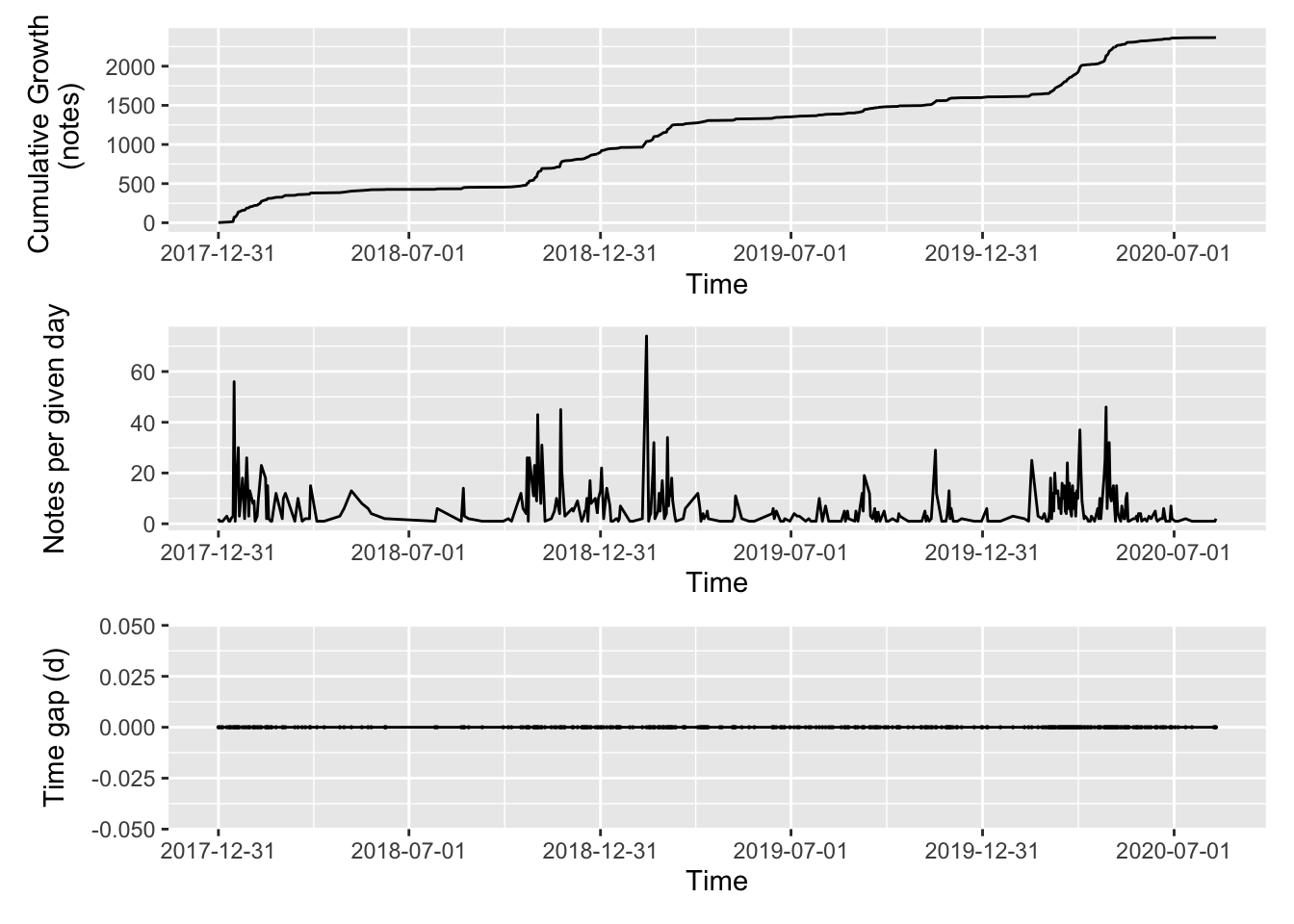

Text analysis

There are also powerful tools for text analysis that I rarely use, but figured this was a good time to try them out. The excellent book (free) Text Mining with R got me up and running very quickly.

Here I look at some words by frequency from the titles and also create a word cloud. There is a lot more one can do to try to find connections between words and all kinds of stuff, but I’ll have to save that for latere.

library(tidytext)
library(wordcloud)

data_table$titles <- titles #add titles to data table

text_data <- data_table %>%
  unnest_tokens(word, titles) 

word_freq <- text_data %>%
  count(word, sort = TRUE) 

nlevels(data_table$entries)

## [1] 340

word_cloud <- word_freq %>%
  with(wordcloud(word, n, max.words = 100))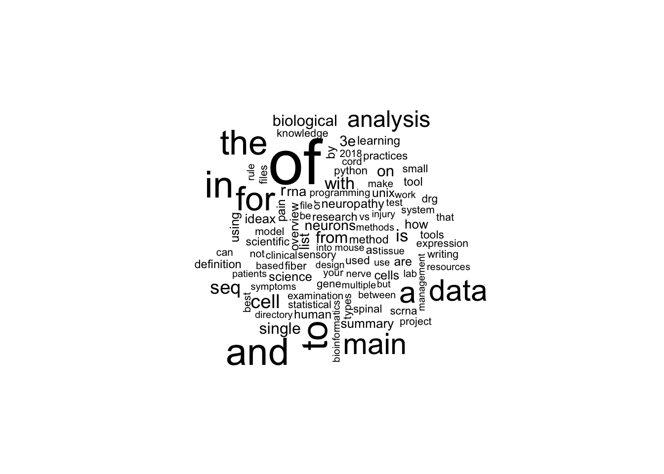

This represents about two year’s worth of serious work with my ZK. It’s satisfying to see the growth and progress over the long term.

Some initial insights:

I’ve done some stuff! The archive has been growing steadily over time.
I have periods where I add a lot more than others. These correspond to periods in my career where I have more time to engage the ZK. When I’m clinical I don’t have much time to add to the ZK. Also, that flat line in mid 2018 corresponds to when I was writing my PhD thesis and wrapping up grad school. I wasn’t adding much then.
- But then in late 2018, when I was relaxing during my 4th year of medical school, I added a bunch more notes.

Try it out yourself

If you’d like to use this for your own ZK visualization, just copy the code into an R markdown document and run it yourself. Make sure to change the directory for where your ZK is.

What other kinds of analyses would you want to see?